Periods
The most important parameter that the model produces is the spot period as it is the crucial variable in determining differential rotation. While the model was very proficient at determining the period I discovered that spot periods tend to persist over long strecthes of time. This was unexpected because spots on the Sun rarely last for more than 30 days but the stars in my sample had spots persist for hundreds of days! This in itself is a significant scientific discovery but I decided to play around with it a little more to see what else I could learn.
The first step was to find a quick way of analyzing multiple spot frequencies at once for long stretches of time. To achieve this I used Fast-Fourier Transforms (FFT) to analyze the lightcurves, this proved to be effective at determining the two strongest frequencies in the lightcurve. I also used a Lomb-Scargle periodigram which basically modeled the data with a simple sin function at reported the two most significant periods. The two techniques produced equivalent results so I performed both types of analysis to verify their intergrity.
Synodic Periods
With the dominant periods in hand I could now analyze the data and see what interesting trends came out. As I mentioned earlier my stars displayed spot periods that lasted in the hundreds of days, as opposed to 30 on the Sun. Since I had two frequencies (or periods) to work with I therefore had the history of two spots to work with. It is then possible to predict future behavior of these periods by considering their synodic period (Psyn) or the beat frequency (fb) which I sometimes used instead:
The synodic period is typically used in orbital mechanics to determine when two planets in orbit around a star, with different periods, will return to their original orbital configuration. With star spots, this equation can be used to predict when two spots with different rotation periods will return to a predetermined configuration. There are two basic starspot configurations to consider 1) when the spots are aligned in longitude and 2) when the spots are in opposite hemispheres. When the spots share a longitude the lightcurve shows the greatest change in flux, however the data does not suggest that two spots are present and the model fails. When the spots are in opposite hemispheres the lightcurve does not display much variation and the model struggles to find solutions. The best times to model are of course during the intervening periods of time, which is fortunately most of the lightcurve. Below is a sample of a lightcurve showing these types of scenarios.
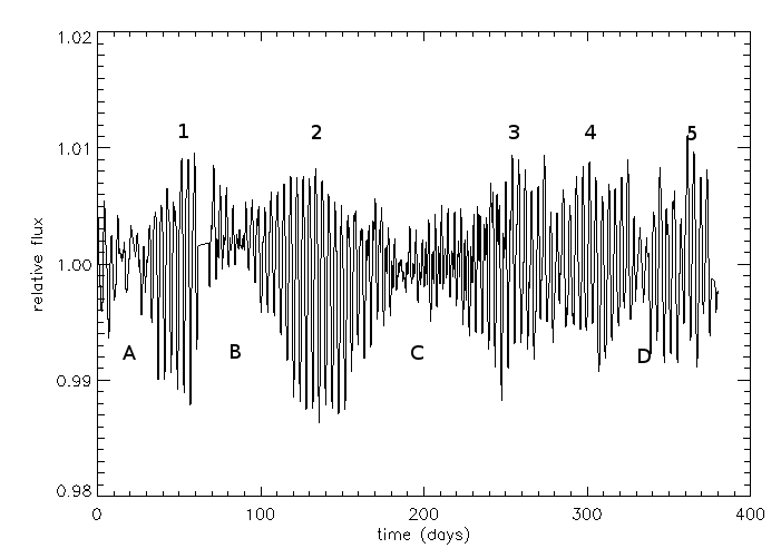
An example of synodic points from KIC 6607150. The numbered points indicate where the spots have similar longitudes. The lettered points indicate where the spots have the greatest difference in longitude. Since more than two spots are present, the spots are constantly changing in size, and differential rotation is present, the spacing of aligned and non-aligned spots is not the same.
Back to my homepage